1. Related methods
There are two other popular methods in the cognitive neuroscience literature which provide alternative solutions to the problem of individual variability: individualized parcellations and Representational Similarity Analysis (RSA). Although not the focus of this site, we briefly contrast these methods with functional alignment to provide a clearer understanding of what functional alignment entails.
1.1. Contrasting anatomically-based alignment
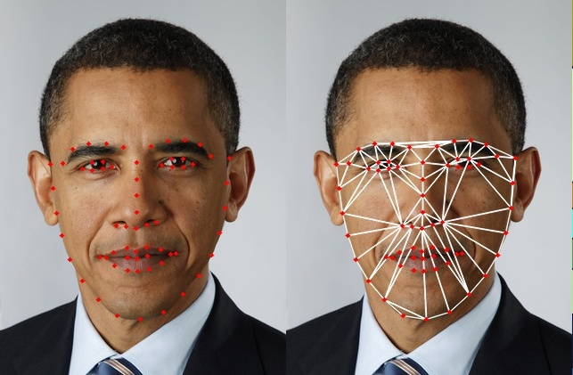
A relevant analogy here—originally suggested by Jack Gallant—is to the idea of face averaging. Much like sulci and gyri in MRI data, faces also have relevant landmarks (e.g. eyes) that can be used to generate a mapping between individual’s faces.

Fig. 1.3 Identifying relevant facial landmarks using OpenCV. With thanks to Satya Mallick.
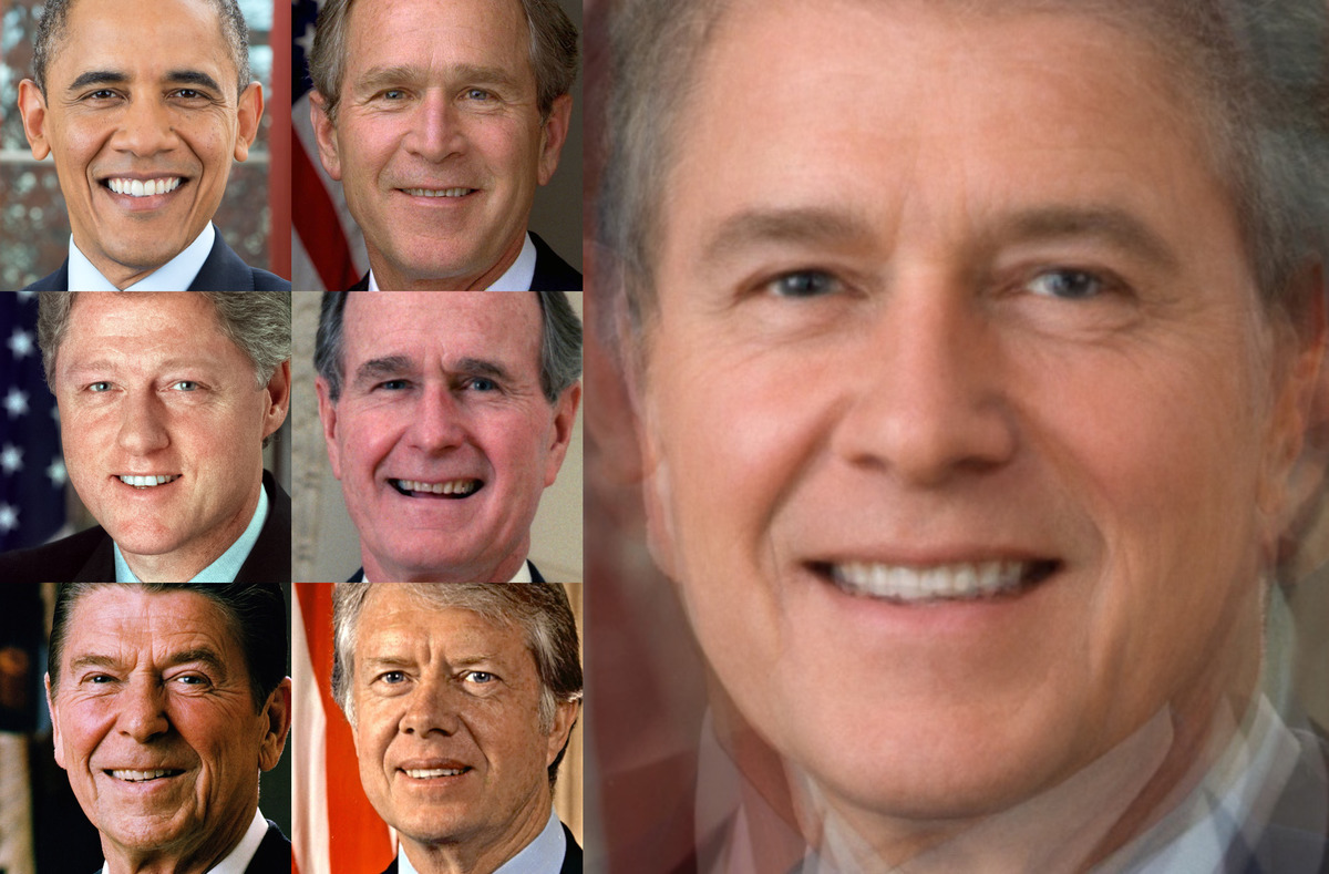
By using these landmarks, we can identify relevant internal structure within an individual’s face; for example, the distance between their eyes. Importantly, because these landmarks are shared across faces, we can generate a mapping between different individual’s facial structures. These mappings can then be used to bring one or more faces into alignment, where they can then be averaged, as shown in Fig. 1.4

Fig. 1.4 An average face from six US presidents, generaged using OpenCV. With thanks to Satya Mallick.
The resulting composite or “average face” retains important structure that is consistent across individuals, but this structure is largely defined by the chosen landmarks. This means that idiosyncratic information—particularly information that is not represented in the original landmarks, such as their hairline—is not well-represented in the composite face.
1.2. Individualized parcellations
High-dimensional neural recordings, such as those achieved through fMRI, measure hundreds of thousands of voxels over hundreds of time points. Computationally, working with this data thus demands some kind of dimensionality reduction. Although many forms of dimensionality reduction have been explored, perhaps the most popular method involves parcellating the brain into a set of functional regions.
This method has a strong sense of biological validity, as we know that the brain shows cytoarchitectonic and functional differences across both cortex and sub-cortex. Although functional parcellations can be directly estimated from an individual’s fMRI scans, variability in their localization makes inter-subject comparison difficult. Many investigators, therefore, choose to rely on canonical parcellations derived from a different group of participants, such as the Schaefer or BASC parcellations.
Because these are group-averaged parcellations, however, we now have the opposite problem–that these parcellations do not appropriately reflect individual-level functional structure! As a result, new methods are being actively developed to “individualize parcellations.” That is, to take a canonical parcellation and alter the spatial extent or localization of its parcels such that it better reflects individual-level organization while still being comparable across the group.
Although the intuition behind individualizing parcellations can be viewed as a form of functional alignment, there is one large conceptual difference. When we parcellate fMRI data, we know that this is a useful form of dimensionality reduction. It is unlikely, however, that the identified areas reflect “true” functional modules in the brain. This requires a much higher evidence-threshold, such as converging cytoarchitectonic boundaries. By individualizing functional parcels, we implicitly agree that we expect this set of parcels to exist across all individuals. It may be possible to describe the data using the set of parcels, but this does not guarantee that these parcels in fact exist across individuals or that they reflect the true data-generating process.
Rather than using pre-established parcels as their starting point, functional alignment methods use the individual functional units. In the case of fMRI data, therefore, alignment transformations are computed directly on the voxels. Functional alignment can be computed within a parcel, and this serves to regularize the resulting transformation. There is no assumption however–implicit or otherwise–that fMRI data can be well-described by a given parcellation.
1.3. Representational Similarity Analysis (RSA)
Much like functional alignment, RSA focuses on comparing representational geometries across subjects. RSA does this, however, in service of a representational model. That is, we have particular stimuli or stimulus classes which are chosen by the experimenter to reflect putative properties of the brain’s functional organization.
For example, we could consider how animacy vs inanimacy is differently encoded in a given cortical region. We would present many animate or inanimate stimuli, and use these stimuli to define our representational geometry. We could then compare this labelled representational geometry with an exisiting representational model, or with data collected using the same paradigm in a different modality such as behavioral reports.
Functional alignment does not have the same reliance on stimuli. Ideal functional alignment stimuli are those which richly sample functional space (such as a Hollywood movie) rather than stimuli which precisely align to an investigator’s hypothesis. As a result, functional alignment methods do not provide a clear path to representational models, even though–like RSA–they involve examining individual-level representational geometries.
1.4. Constraining functional alignment to local neighborhoods
Since functional alignment is not guided by anatomical landmarks, considering a large number of voxels can generate biologically implausible transformations. For example, we may maximize distribution similarity while aligning voxel activity from one participant’s visual cortex to another participant’s prefrontal cortex. To avoid this, we can constrain the voxels included in calculating each functional alignment transformation to smaller, local neighborhoods.
A relevant neighborhood might be defined by an a priori region of interest (ROI). That is, a researcher may have identified a relevant patch of cortex through functional localizers or anatomical tracing. They can then only consider voxels within this ROI and functionally align their activity across participants.
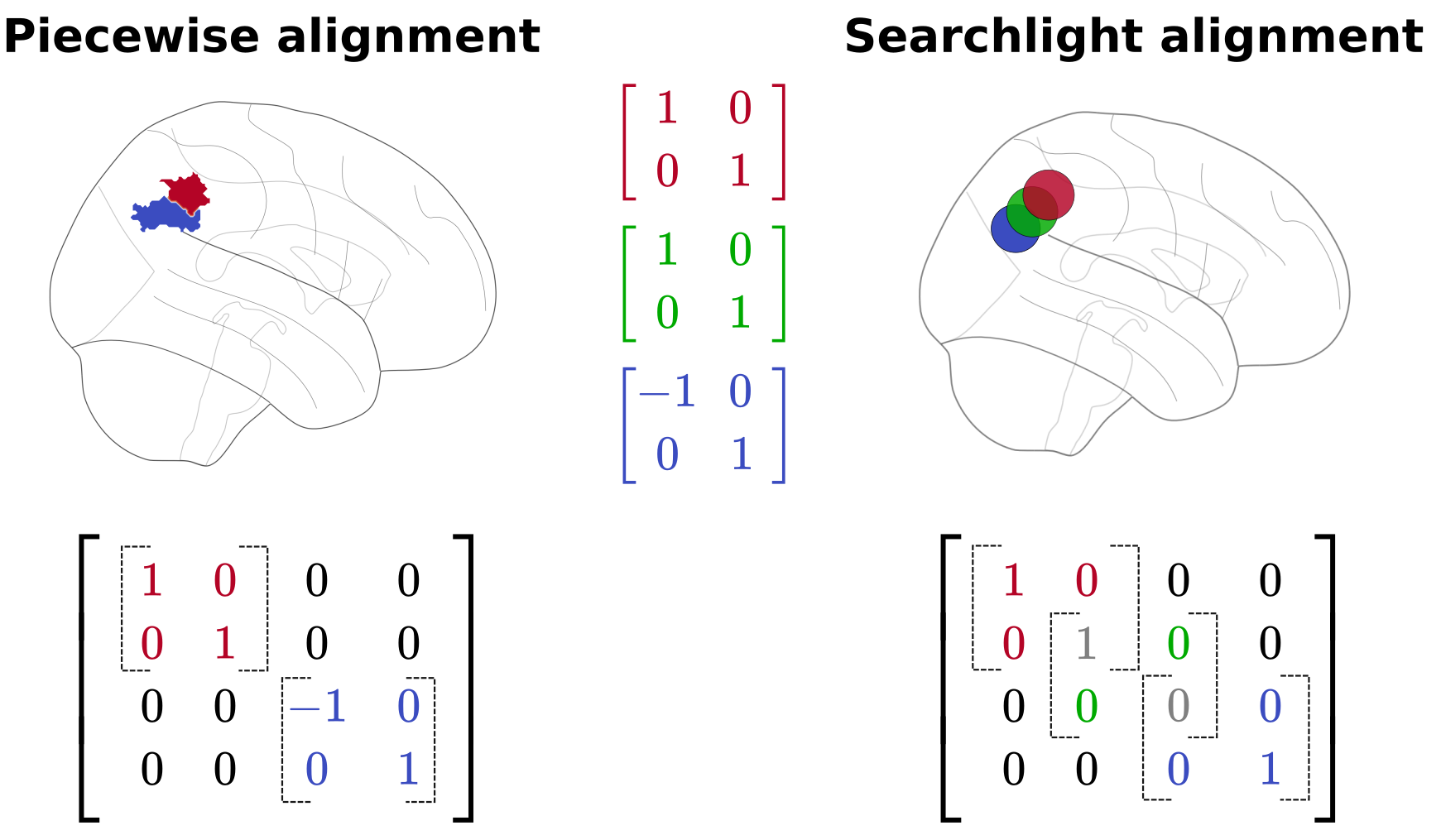
To generate a whole brain transformation, however, we must define many more local neighborhoods. There are two primary strategies to do so. The first is through a deterministic or non-overlapping parcellation. This can be considered as an extension of the ROI-based approach, in that we now have as many ROIs as there are parcels. Transformations are calculated separately for each parcel and then aggregated into a larger whole brain transformation matrix.
Alternatively, we can define our local neighborhoods using a searchlight approach. Here, a searchlight is a small sphere of defined radius that we can iterate through a brain volume. Importantly, the centroids of each searchlight are selected such that the spheres slightly overlap. When generating an aggregated transformation, then, this overlap must be accounted for in the transformation itself; for example, by averaging or summing the calculated transformation from two overlapping searchlights. You can see an example of these different local neighborhood methods in Fig. 1.5.

Fig. 1.5 Two different methods to constrain functional alignment transformations: non-overlapping parcels from a deterministic parcellation or partially overlapping searchlights.
Importantly, when functional alignment transformations are aggregated using the searchlight methods, the final transformations are no longer guaranteed to have the same properties as the initial, unaggregated transforms. In this work, we therefore assume that functional alignment transformations are calculated in non-overlapping neighborhoods, such as an ROI or a whole brain deterministic parcellation.
