5. Canonical Correlation Analysis
Canonical correlation analysis (CCA) is a form of multi-view learning where we have paired observations or “views” that contain complementary information on an underlying (or “latent”) process. CCA learns two linear projections —one for each view— such that the projected data points are maximally correlated. That is, the paired data points are projected into a shared space such that they lie as close as possible to one another. These linear projections can be considered to reflect features of the structure of the data and may thus be useful for downstream prediction tasks.
Another perspective on CCA comes from considering it as a prediction task itself. Specifically, because CCA assumes that each set of observations is dependent on one or more shared latent variables, we could learn the relevant linear projections on a subset of the data and apply them on a held-out portion of the data set.
In this post, we’ll consider the mathematics of CCA to guide our intuitions about the method. Departing somewhat from classical CCA walk-throughs, we’ll focus on regularized CCA and its usage in predictive contexts. This focus will allow us to consider applications of regularized CCA as a functional alignment method in both the neuroscience and artificial intelligence literatures.
5.1. Formalizing the problem
Suppose we have two mean-centered data matrices \(X_a \in \mathbb{R}^{n \times p_1}\) and \(X_b \in \mathbb{R}^{n \times p_2}\), where \(n\) is the number of samples, and \(p_1, p_2\) are the number of units for each network. We can say without loss of generality that \(p_1 \leq p_2\).
Because we consider these two sets of activation patterns to be paired, we can note the \(i\)-th sample as two row vectors, \((\mathbf{x}_a^i, \mathbf{x}_b^i)\) with dimensionality \(p_1\) and \(p_2\), respectively. We thus have \(n\) paired observations.
By applying linear projections to our original \(X_a\) and \(X_b\) matrices, we can then generate a pair of canonical components or canonical variables. We denote these as \(\mathbf{z}_a \in \mathbb{R}^n\) and \(\mathbf{z}_b \in \mathbb{R}^n\) such that:
Our goal is to learn transformations that maximize the correlation of these canonical variables:
This is equivalent to finding the minimum angle \(\theta\) between them:
This geometrical interpretation is the view reflected in Fig. 5.1.
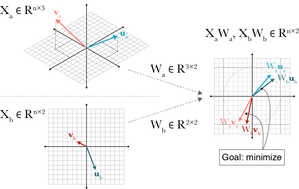
Fig. 5.1 A visualization of canonical correlation analysis. Let \(n=2\) be the number of observations. Two datasets \(X_a \in \mathbb{R}^{n \times 3}\) and \(X_b \in \mathbb{R}^{n \times 2}\) are transformed by projections \(W_a \in \mathbb{R}^{3 \times 2}\) and \(W_b \in \mathbb{R}^{2 \times 2}\) such that the paired embeddings, \((\mathbf{v}_a, \mathbf{v}_b)\) and \((\mathbf{u}_a, \mathbf{u}_b)\) are maximally correlated with unit length in the projected space. Figure from Gregory Gundersen [Gundersen, 2018].
5.1.1. Working with well-sampled data
We can start by looking at the empirical covariance matrices for each of our sets of observations.
We denote the covariance matrix between data sets \(X_i\) and \(X_j\) for \(i, j \in \{a, b\}\) as \(\mathbf{C}_{ij}\). Then, the covariance and cross-covariance matrices for \(X_a\), \(X_b\) can defined as:
With these, we can define the composite or joint covariance matrix as:
From our original definitions of \(\mathbf{z}_a\) and \(\mathbf{z}_b\), we can see that:
Substituting in Equation (5.3)—and keeping in mind we have mean-centered our data such that that our canonical variables have unit length–we can re-write Equation (5.1) as:
This equation can be solved using eigenvalue decomposition, as proposed by [Hotelling, 1936]. For a detailed walk-through of this solution, see Fig. 5.1.
5.1.2. Considering small sample sizes
In research applications, we are often not working with well-sampled data sets. In this case, we can return to (5.2) and ask: what we can do when our empiricial covariance matrices are unlikely to reflect our theoretical covariance matrices?
We know from [Pezeshki et al., 2004] that if our \(n\) observations are less than the sum of \(p_1\) and \(p_2\), then \((p_1 + p_2) − n\) canonical correlations will be equal to one. This means these canonical correlations do not carry any information about their true population values.
Why might this be?
At the same time, a key question in any correlation analysis is how many correlated signals there are. If we had access to the population canonical correlations, we could simply count the number of nonzero ki’s.
This implies that the sum of the ranks of the two data matrices determines the minimum number of data samples (sample support) required to estimate the theoretical canonical correlations
This projection is particularly useful when the two sets of observations have different dimensionality. In neuroscience, these complementary views are therefore often examined as brain-behavior correlations. However, CCA can be used in any multi-view learning context.
The goal of this post is to demonstrate the application of CCA to problems from the functional alignment literature. This literature encompasses both neuroscience and artificial intelligence, so to be broadly inclusive we will generally refer to to-be-aligned activations as occurring in networks without denoting whether these networks are biological or artifical.
As an initial motivation, we can consider that two networks activity patterns reflect two different views of a shared representational geometry.
One important note is that, so far, we have only denoted one pair of canonical variables. In principle, however, we could define multiple pairs of canonical variables, up to \(p_1\) pairs. Each of these pairs should be orthogonal, however, such that
for all \(j < i\).
import numpy as np

x_a = np.random.rand(1, 2)
x_b = np.random.rand(1, 3)
5.2. References
- 1
Gregory Gundersen. Canonical correlation analysis in detail. https://gregorygundersen.com/blog/2018/07/17/cca/, July 2018.
- 2
Harold Hotelling. Relations between two sets of variates. Biometrika, 28(3-4):321–377, December 1936.
- 3
A Pezeshki, L L Scharf, M R Azimi-Sadjadi, and M Lundberg. Empirical canonical correlation analysis in subspaces. In Conference Record of the Thirty-Eighth Asilomar Conference on Signals, Systems and Computers, 2004., volume 1, 994–997 Vol.1. November 2004.