2. Ridge Regression
Let’s say that you’d like to predict one distribution Y from the other distribution X. In previous work such as Tavor, Jones, Mars, Smith, Behrens, and Jbabdi [2016], we’ve seen this method used to predict one task condition (such as a working memory task) from another (such as resting-state) within the same participant.
We can do so by predicting \(Y\) as a weighted combination of information from \(X\). The corresponding model would look something like this,
where we have two unknowns:
\(\beta\) refers to a matrix of weights, one for each voxel, and
\(\epsilon\) refers to a matrix of noise, i.e. any part of \(Y\) that you can’t predict from \(X\).
2.1. Learning the \(\beta\) weights
Our goal is to learn the \(\beta\) weights that minimize our “noise” or error values, \(\epsilon\). Ordinary Least Squares (OLS) is an ideal approach to solving this regression in that it provides the Best Linear Unbiased Estimator (BLUE). A nice introduction to OLS is available from Mumford Brain Stats.
Unfortunately, using OLS regression tends to overfit to a given data sample, meaning that our learned \(\beta\) values will not generalize well to new data. This is important, as we do not want to learn mappings between only two sets of samples (i.e. one run each of resting-state and task). Instead, we want to learn mappings that generalize to new samples collected under the same conditions. We therefore need to reduce how much we’re overfitting to our training samples.
To do so, we can modify the learnt \(\beta\) weights using a set rule. Although many different rules are possible, here we’ll use “ridge,” from which ridge regression gets its name. This is also known as an L2 penalty.
2.2. Improving performance with an L2 penalty
The simplest way to describe ridge regression mathematically is including a penalty on the size of the weights in the loss function. Specifically, ridge regression penalizes the sum of the squared weights, leading to a new and improved loss function that we’ll call \(\mathcal{L}_{ridge}(\beta)\):
or, in fancy linear algebra terms:
The first term on the right hand side of this equation is the same squared error loss that we used before for OLS. The second term is the sum of the squares of all the weights in \(\beta\), multiplied by a scalar variable \(\lambda\) that we will call the ridge coefficient
The ridge coefficient \(\lambda\) determines the strength of the regularization that’s applied in ridge regression:
If you give \(\lambda\) a large value, then the penalty term will be big relative to the loss, and the resulting weights will be very small. (In the limit of very large \(\lambda\) you will force the weights to be almost exactly zero!)
If you give \(\lambda\) a small value, then the penalty term will be small relative to the loss, and the resulting weights will not be too different from the OLS weights. (In the limit of \(\lambda \rightarrow 0\), the penalty term will be zero and you’ll get back exactly the OLS solution!)
To get the ridge regression weights, \(\beta_{ridge}\), you minimize the ridge loss function. We don’t need to go through the full derivation of the solution (though it’s pretty fun, and easy to do based on the matrix calculus we did for the OLS solution!), so let’s just take a look at the answer:
Compute \(R\) s.t. \(|| XR - Y ||^2 + alpha ||R||^2\) is minimized with CV.
2.3. Implementing directly in nilearn
There’s an example in the Nilearn gallery that uses ridge regression to predict fMRI activity from visual stimuli.
We can lightly adapt this example to predict fMRI activity in one condition from another condition.
from sklearn.linear_model import RidgeCV

R = RidgeCV(alphas=self.alphas, fit_intercept=True,
            normalize=False,
            scoring=sklearn.metrics.SCORERS['r2'],
            cv=self.cv)
R.fit(X, Y)
