2. Distribution alignment
With neuroimaging data, we usually make inferences across subjects by creating a mapping between each subject’s neuroanatomy; this is typically done by normalizing their anatomical (T1-weighted) MRI scan to a standard template such as the MNI152. We can then look at similarities across individuals in this standardized space, assuming that voxel \(X_1, Y_1, Z_1\) corresponds across individuals.
Assuming we’d like to work with voxelwise data, we would then extract the activity time courses for all given voxels of interest, such that we had graphs of voxel activity over time. We could then compare the similarity of these time courses using techniques such as correlation. To compare across individuals or brain states, then, we would compare summary-level statistics from e.g. network analysis.
As shown in Fig. 2.1, our question then is how best to find correspondence between two (or more) unique functional spaces.
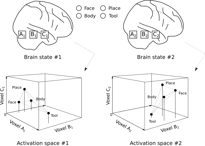
Fig. 2.1 The locations of four protoype points within the voxelwise activation spaces of two brains. Figure adapted from Churchland [1998].
2.1. Formalizing the problem
Suppose we have two data distributions, \(X\) and \(Y\). These distributions may come from voxel activity time series sampled from two different participants or from the same participant in two different psychological tasks.
Each distribution contains a series of \(n\) observations, such that \(X = \{\mathbf{x}_1, \ldots, \mathbf{x}_n\}\) where \(\mathbf{x}_i \in \mathbb{R}^p\).
For fMRI data, then, \(n\) would be the number of time points sampled, while \(p\) is the number of voxels considered.
To deal with these equations more easily, we’ll need to stack the values of \(x\) and \(y\) into matrices. Let’s define those matrices like this:
Now we have two matrices, where each matrix represents one of our two distributions \(\mathbf{X} \in \mathbb{R}^{n \times p}\) and \(\mathbf{Y} \in \mathbb{R}^{n \times p}\).
For some methods, we will enforce that every distribution has exactly the same number of voxels \(p\). Other methods will allow the number of voxels to vary across distributions. When variable voxels are allowed, we will denote the number of voxels as \(p_1\) or \(p_2\), corresponding to the relevant distribution.
Note
Some latent factor models reduce the number of dimensions using an initial decomposition. The idea is that there may be several latent factors supporting voxel-level activity patterns, and we can therefore capture relevant information even in a lower dimensional space.