3. Procrustes alignment
Originally introduced in [Schönemann, 1966], Procrustes analysis is a form of statistical shape analysis which focusses on comparing the geometry of two objects or data sets. Although it may seem unusual to think of distributions in terms of geometry, this makes more sense when we consider the distributions as point sets in some activation space.
Because we assume a known correspondence between these two distributions, we can directly compare the \(i\)-th sample across \(X\) and \(Y\). The goal in Procrustes is to find a single orthogonal transformation that minimizes the sum-of-squares distances between all \(n\) \(X\), \(Y\) pairs, thereby minimizing the total distance between the distributions.
3.1. Orthogonal Procrustes
Our goal, then, is to find linear transformations that minimize the total distance between the two distributions. By further assuming that each distribution has exactly the same number of voxels \(p\) measured over the same \(n\) observations, we can consider that we are comparing two shapes with a known one-to-one mapping; i.e. the \(i\)-th voxel in the \(X\) distribution corresponds to the same voxel index in the \(Y\) distribution. Procrustes analysis allows us to align the shapes as closely as possible through linear mapping and to quantify how much they differ after this alignment.
3.1.1. Formalism
import numpy as np

X = np.random.rand(20, 100)
Y = np.random.rand(20, 100)
For our two distributions \(\mathbf{X} \in \mathbb{R}^{n \times p}\) and \(\mathbf{Y} \in \mathbb{R}^{n \times p}\), Procrustes solves the following minimization:
Where \(|| \cdot ||_F\) indicates the Frobenius norm, which corresponds to the elementwise Euclidean distance.
from scipy.linalg import svd

A = Y.T.dot(X)
U, s, V = svd(A, full_matrices=0)
R = U.dot(V)
sc = s.sum() / (np.linalg.norm(X) ** 2)
3.1.2. Implementation
Optimized implementations are available in scipy.linalg.orthogonal_procrustes.
from scipy.linalg import orthogonal_procrustes

R, sc = orthogonal_procrustes(X, Y)
3.2. Generalized Procrustes
Generalized Procrustes analysis differs from Procrustes analysis in two ways. First, generalized Procrustes includes both the orthogonal transformations of Procrustes (i.e., rotations and reflections), as well as additional scaling and translation transformations. Second, generalized Procrustes can be applied to more than two shapes through the iterative use of a reference shape.
We can formally express the generalized Procrustes problem as:
3.2.2. Implementation
Optimized implementations are available in scipy.spatial.procrustes.
from scipy.spatial import procrustes

mtx1, mtx2, disp = procrustes(X, Y)
3.3. References
- 1
Peter H Schönemann. A generalized solution of the orthogonal procrustes problem. Psychometrika, 31(1):1–10, March 1966.
